How To Make A Simple Website Ripper With Google Sheets

Ripping a website’s source code is the starting point for many, many SEO tasks. Whether you’re verifying updates, checking for open graph, checking for schema markup, or trying to figure out which pages are missing that oh-so-important CSS file, if you’re in the SEO field – at some point, you’re going to be digging through source code. If you’ve never done this before, imagine going to each page on a site, right-clicking, selecting “View Page Source”, and the Control-F searching for some word or snippet in the code. What a pain in the ass. Good thing there’s a better way. Let’s power up Google Sheets and dive in.

The magic of ImportDATA

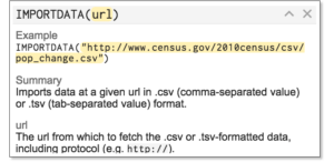
ImportDATA is a function in Google Sheets. It’s a lot like other functions you may have seen in spreadsheets, except that it’s some kind of freaking magic. If you’ve used spreadsheet applications like Google Sheets or Excel, you might have used things like SUM(Range), which takes an input of cells and performs an action on them – in SUM’s case, adding them together and giving you the result. ImportDATA works in a very similar way, just with a way more magical function.

ImportDATA lets you specify a URL, and it will pull back the URLs source code. You read that right. Google basically built a website ripper function, and you don’t need to do anything except tell it what URL to rip:

=importdata("https://www.ranktank.org/learn/")

Yes, it’s really that simple. Let’s give that above call a whirl, and see what happens when we run the formula on my favorite URL: https://www.ranktank.org/learn/

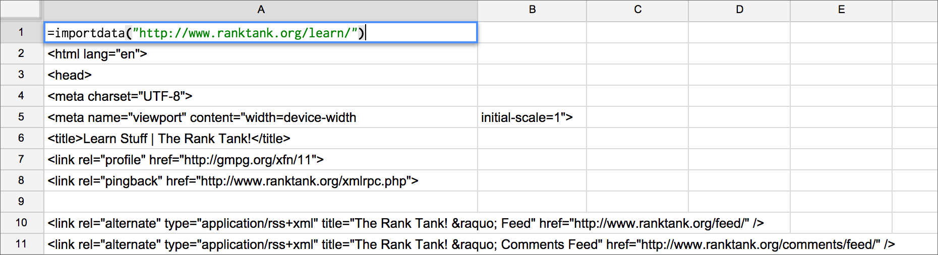
Woah. That’s pretty awesome. That simple formula pulled all of the URL’s source code into the spreadsheet. Like freakin’ magic.

Building it into a bulk tool

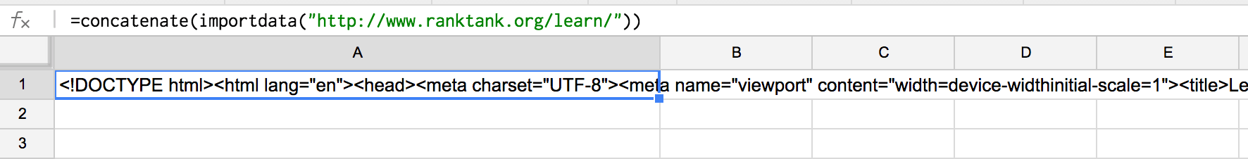
As you could see in the screenshot, ImportDATA pulls back all of the code for the page in a big list of stuff broken out into multiple cells. However, what we really want to do is make a tool that pulls in code from a whole list of URLs. We’re going to have to get the code to come back in a single cell. Luckily, there’s a formula for that: Concatenate. This formula is meant to combine an array of data into one string… an array like the one that ImportDATA returns!

=concatenate(importdata("/category/learn/"))

Adding Concatenate wrapped around our ImportDATA call does exactly this! All of the ImportDATA returned code is neatly tucked into a single cell.

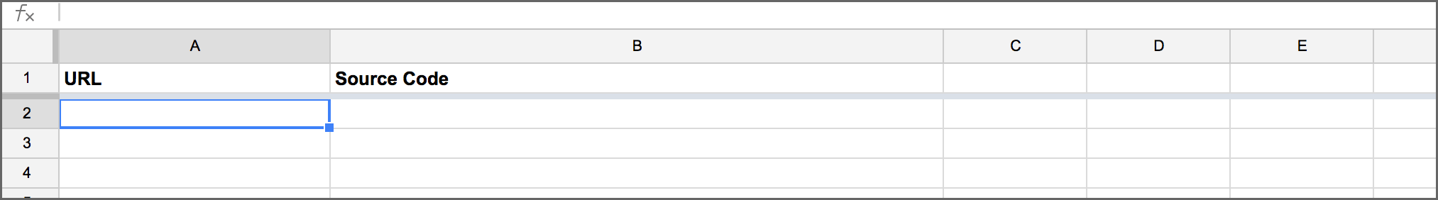
Sweet. Now we have to build a way to paste in a bunch of URLs and have the formula run automatically on them. It’s way easier than it sounds, and I bet you’ve done this before: we’re just going to run ImportDATA on a cell name! Let’s set up column A as the URL column, and column B as the Source Code column.

Then, we’ll pop a bit of code into cell B2. It’s going to be basically the same as the code we made above, but instead of a URL, we’re going to use A2 to reference the cell where the URL will be pasted.

=concatenate(importdata(A2))

Next, we’re going to fill column B down. Simply select cell B2 (where you put the above formula), and then select all the way down to the last cell in column B. Then, on your keyboard, press the key combo Control-D. This will fill the formula down in a series, so each cell in column B will reference the right cell next to it in column A.

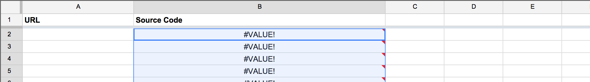
Now you’ll notice that it’s a bit ugly right now – since there aren’t any URLs in column A, all of the cells in column B have the error message #VALUE.

Even though this won’t affect the functionality of the sheet – we can actually paste URLs in column A right now and it will work – let’s clean this up a bit. Because, you know, we’re classy? Let’s change the formula in cell B2 to the following, and then fill it down:

=if(a2="","",concatenate(importdata(A2)))

All we did there was add a check to see if cell A2 was blank using an IF statement, or as your computer dweeb friends might call it, a conditional. It’s pretty straightforward. It’s basically doing this:

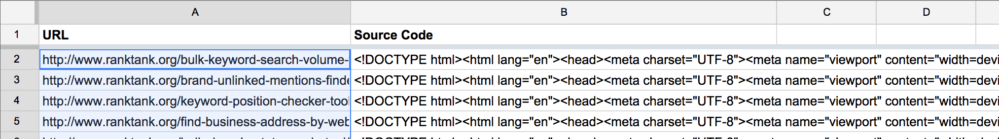
It’s so simple. Woot. We now have a fully functioning tool! You can paste a list of URLs in column A, and column B will return the source code! Oh, and if you want to clean it up even further, we can stop it from making HUGE scrolling cells with all of the source code by removing line breaks from the returned code. We’re can just wrap a formula called Substitute around our stuff, and substitute char(10) for “” (char 10 is the code for line breaks):

=if(a2="","",substitute(concatenate(importdata(A2)),char(10),"")

Sure that formula might look complicated now, but if you’ve followed along, you’ll see that it’s pretty understandable. And look how cool and clean our sheet is!

Here’s a link to the completed sheet. If you want to use it, do File -> Make a copy in Google Sheets to save it to your own Google account.

I hope this helps you out! I also really hope this opens your eyes up to the HUGE possibilities of crazy shit you can do with Google Sheets! Imagine using this to check if pages on a site have been updated by automatically checking each page’s source code in bulk, or parsing a website’s sitemap to pull in all of the URLs, and getting the source code for all of them…

If you have any questions, or if you’ve built something cool out of this, hit me up in the comments!